PDF version
Cite
H. França, H. Schubert, O. Versolato & M. Jalaal, Laser-Induced Droplet Deformation: Curvature Inversion Explained from Instantaneous Pressure Impulse, J. Fluid Mech., 1020, A21 (2025). DOI (OA): 10.1017/jfm.2025.10665
Context
Extreme‑ultraviolet (EUV) nanolithography relies on shaping a liquid tin microdroplet into a thin sheet with a nanosecond “prepulse”, then ablating that sheet with a second pulse to create the EUV‑emitting plasma. The fluid dynamics between those two laser hits matter: sheet curvature, thickness, and expansion rate all feed directly into plasma formation and light yield. A persistent puzzle has been that many experiments produce forward‑bending sheets (curving away from the incoming beam), whereas standard theories—driven by Gaussian pressure impulses—predicted the opposite. A recent JFM paper by França et al. resolves this discrepancy by introducing a raised‑cosine pressure impulse and a single width parameter that governs when the sheet flips from backward to forward curvature.
At a glance
Key idea: The kurtosis of the instantaneous pressure impulse controls the sign of the tin sheet’s curvature. Low‑kurtosis (raised‑cosine) impulses can bend the sheet forward; Gaussian impulses cannot.
Switching knob: A dimensionless width (W) of the pressure impulse: curvature flips sign near (
). Practical proxy: (
) correlates with the beam‑to‑drop size ratio ( ); curvature inversion occurs experimentally at ( ).
What’s new?
A one‑parameter impulse that explains both curvature regimes. The authors propose a raised‑cosine surface‑pressure impulse (
A predictive diagnostic from the initial velocity field. By solving Laplace’s equation for the instantaneous pressure inside the drop and extracting the initial velocity via a Legendre‑series construction, the team shows that the angle of maximum radial velocity (
How did they show it?
Direct numerical simulations with experimental anchoring. Using a VOF solver (Basilisk C) at very high resolution (quadtree level 14; minimum cell (
Mapping (
Why does the raised cosine work?
The curvature outcome is set by where the impulse deposits momentum:
-
Gaussian (mesokurtic): widening the peak also lengthens the tails; the pressure effectively “wraps” the drop, leaving the region of strongest radial push behind the equator (
). Sheets bend back toward the source. -
Raised cosine (platykurtic): broad peak, short tails. For sufficiently large (
), the direction of maximum radial expansion shifts beyond the equator ( ), driving the rim forward and producing positive curvature. The sign flip emerges around ( ). (See table 1 and the ( ) analysis.)
Kurtosis as a design heuristic
Seeking forward curvature? Favor low‑kurtosis impulses that are wide‑peaked but short‑tailed. The raised cosine is one smooth, tunable option—but other low‑kurtosis shapes should behave similarly.
What does this mean for EUV source design?
-
A controllable knob for sheet morphology. Because (
) correlates with optical focusing, curvature can be selected via the beam diameter relative to the droplet, with the transition near ( ). This provides a practical handle to realize forward‑bending sheets—beneficial for subsequent plasma shaping and possibly for more uniform ablation by the second pulse. (See the regime map and time‑lapse comparisons.) -
Thickness distribution matters. Simulations indicate that larger (
) (unfocused, low‑kurtosis impulses) yield sheets with more uniform thickness across the span—attractive for even energy deposition. (Snapshots in figure 6 show this trend.)
Quick‑design recipe (from the paper’s workflow)
Choose an impulse with low kurtosis (e.g., raised cosine) and estimate (
) from the intended ( ) using ( ). Compute the (
) velocity field and locate ( ).
• If () → expect forward curvature.
• If () → expect backward curvature. Only then run full DNS to refine thickness and late‑time rim dynamics.
Caveats and open questions
Despite the strong agreement on curvature, two gaps remain—useful pointers for future work:
-
Expansion vs. propulsion speed. In the simulations, positive‑curvature cases (large (W)) systematically produce low expansion‑to‑propulsion ratios (
), whereas experiments sometimes show fast expansion and positive curvature. Closing this gap likely requires more faithful modeling of the laser–plasma drive (e.g., via radiation‑hydrodynamics) or impulse shapes beyond the pure raised cosine. -
Ambient medium and late‑time rims. Numerically, the surrounding “vacuum” must be given a tiny but finite density (e.g.,
), which introduces slight drag and affects rim formation at late times; sensitivity sweeps suggest curvature trends are robust, but detailed rim physics—and any 3D asymmetries—are outside the axisymmetric model.
Outstanding physics to nail down
Direct experimental inference of the instantaneous impulse profile (ion/charge diagnostics, angular momentum flux).
Multi‑physics coupling (plasma expansion + incompressible hydrodynamics) to reconcile (
) in the forward‑curvature regime. Fully 3D effects and fragmentation (beyond axisymmetry) at the sheet edge.
Perspective
França et al. put curvature control on a firm mechanistic footing: it is the spatial statistics of the impulse—not merely its magnitude—that sets the sheet’s sign and shape. For engineers, the message is actionable: choose beam sizes (and therefore impulses) that place the maximum radial push beyond the equator; for theorists, the link between kurtosis and morphology suggests a compact language to classify laser–droplet interactions across materials and scales. The raised‑cosine model is not the final word on the impulse, but it provides a powerful organizing principle and a practical design rule for EUV source optimization.
footnote
Useful quantities and timescales: (
), ( ), ( ) for tin; typical ( ) and ( ) are ( ).
Source
H. França, H. Schubert, O. Versolato & M. Jalaal, Laser-Induced Droplet Deformation: Curvature Inversion Explained from Instantaneous Pressure Impulse, J. Fluid Mech., 1020, A21 (2025). DOI (OA): 10.1017/jfm.2025.10665 Key details on the impulse definition, (
) diagnostic, ( ) map, timescales, numerical setup, and limitations are summarized above; see in particular the introduction and figures 1–8, Appendix B (ambient effects), and Appendix E (velocity ratio).
Metadata
Author:: Vatsal Sanjay
Date published:: Oct 6, 2025
Back to main website