Lecture 6: Elastic, Viscous and Viscoelastic in Action — Sheets, Bubbles and Drops

PDF version

Download this page as PDF

TL;DR

Lecture 5 gave us one constitutive model, the Oldroyd-B family, whose limits are a viscous liquid, an elastic solid and a Kelvin–Voigt solid. This lecture puts it to work on three free-surface flows from current research: a retracting liquid sheet, a bursting bubble and an impacting drop. We compare material memory and stiffness through the Deborah number (how long the material remembers its deformation, compared with how fast the flow is) and the elastocapillary number (how stiff the material is, compared with surface tension), while the solvent Ohnesorge number measures viscous effects. Drop impact adds the Weber number , which compares the incoming inertia with surface tension. The recurring question is which stress wins: capillary, viscous or elastic.

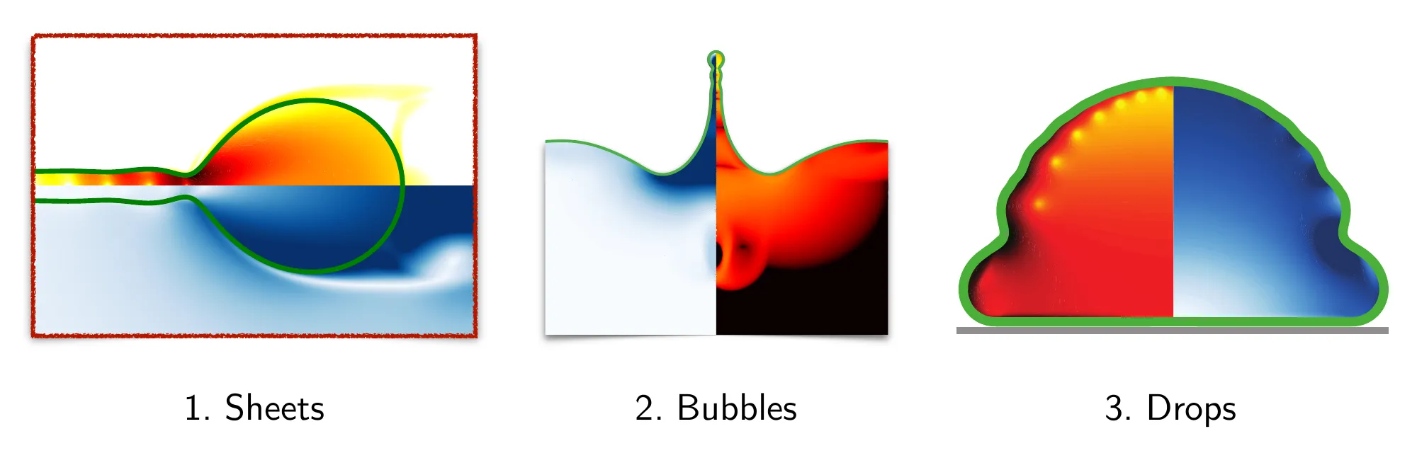The three examples of this lecture, from direct numerical simulations: a liquid sheet retracting into a rim, a bursting bubble launching a Worthington jet, and a drop spreading on a surface.

0) Recap: one model, three limits

In a dilute polymer solution the stress has a solvent part and a polymer part:

Here is the pressure, the solvent viscosity, the strain-rate tensor, the elastic modulus of the polymer network, its relaxation time and the conformation tensor, which measures how stretched the polymers are on average ( at rest). The upper-convected derivative

with , is the rate of change of seen by a material element that moves, rotates and stretches with the flow. The polymer viscosity is .

The limits of the model taught in Lecture 5 are:

• : the polymers relax instantly, , and the material is a viscous (Newtonian) liquid. Keeping the first correction, , so the polymers simply add a viscosity . We use this in §2.
• : the polymers never relax, , and just records the deformation. Starting from a relaxed reference state (), , where is the deformation gradient. The polymer stress is then that of an elastic solid, in parallel with the solvent’s viscous stress: a Kelvin–Voigt solid. Over a deformation time , solvent damping is negligible when , and the response is then purely elastic.

Dimensionless groups

Take a length scale (the sheet thickness , or the bubble or drop radius ), density and surface tension . Measuring time in units of the inertio-capillary time and stress in units of leaves three numbers:

and, writing for the extra stress (the stress apart from pressure), the model becomes

The Deborah number compares the material’s memory with the flow time; the elastocapillary number compares the elastic stress with the capillary stress; the Ohnesorge number compares viscous with inertio-capillary effects.

Two routes to a Newtonian liquid

Both and give a Newtonian liquid, for different reasons. At the polymers relax before they can be stretched (). At the polymers can be stretched as much as you like, but they carry no stress.

1) Sheets: retracting films

1.1 The Newtonian case

A punctured soap film retracts into a growing rim (see the high-speed video of a popped soap bubble). As we saw in Lecture 1.5, the rim moves at the Taylor–Culick speed

with the surface tension of one film–air interface, the film density and its thickness. Following the slides, the film Ohnesorge number is ; the factor two counts the two interfaces, so this is the Ohnesorge number of Lecture 1.5 divided by .

Simulations make the energy budget visible. Of the surface energy released, , about half goes into the kinetic energy of the rim and half is dissipated:

The dissipation is concentrated in the neck where the film joins the rim, and its rate does not depend on the viscosity. Even as we cannot neglect viscous dissipation in the thin film: a vanishing viscosity still dissipates a finite amount of energy, because the velocity gradients sharpen as the viscosity drops. This “dissipative anomaly” is the mathematical version of de Gennes’s inelastic-collision argument. The same simulation framework is used to study films retracting in viscous surroundings (Sanjay, Sen, Kant & Lohse 2022).

1.2 What if the film is viscoelastic?

The “Friday afternoon experiment” in Lecture 1 showed that a polymeric film ruptures differently depending on how quickly it is blown (Tammaro et al. 2018): the timescale of the process matters. To isolate the role of elasticity, take the limit , in which the polymers never relax. At the film still behaves as a viscous liquid. As grows, elastic stresses build up as the film is swept into the rim.

What resists the opening? Picture a circular hole of radius opening in the sheet. The material collected into the rim is stretched in two ways:

• Vertically, as the rim thickens (normal stress ).
• Azimuthally, because each material ring is carried from its original radius out to a larger radius . This is a hoop stretch , and it produces a tensile hoop stress .

Only the hoop stress acts on the radial motion of the rim. With the polymeric hoop stress and the surface tension of each face of the sheet, the momentum balance of the rim reads

The left-hand side is the rate of change of the rim’s momentum; capillarity pulls with per unit length of the rim, and the hoop tension of the stretched sheet pulls back.

To evaluate in the elastic limit we need the deformation, which is set by kinematics alone (Snoeijer, Pandey, Herrada & Eggers 2020). A material point at in the undeformed sheet is mapped to . If the vertical stretching is homogeneous (, with and the undeformed and deformed local thicknesses) and shear-free, volume conservation fixes the map from the thickness profile . For a neo-Hookean (Oldroyd-B elastic-limit) material, with and , so the hoop stress is

The hoop stretch is largest for the material that has travelled furthest, which sits next to the rim. The hoop tension is therefore concentrated near the tip and grows as the hole opens. Comparing the modulus with the capillary stress gives . For stretches of order one, this suggests strong elastic resistance once is of order one, possibly enough to stop the hole from opening. This is a dimensional estimate: the actual outcome also depends on the accumulated stretch and on the geometry of the sheet.

2) Bubbles: Worthington jets in viscoelastic liquids

2.1 Champagne and Worthington jets

A bubble that reaches a free surface bursts. After its cap ruptures, the open cavity collapses and capillary waves converge towards its base. Depending on the bubble size and the liquid properties, this focusing can produce an upward Worthington jet that breaks into droplets. In a glass of champagne these droplets carry the aroma above the glass (Ghabache, Liger-Belair, Antkowiak & Séon 2016). The same process launches aerosol droplets from the sea and from contaminated liquids. So what does a small amount of dissolved polymer do to the jet and its droplets?

The question is not new. Cheny & Walters (1996) compared the Worthington jets that rise after an impact on a liquid pool. For a Newtonian liquid the jet reached about 20 cm; for a Boger fluid (a dilute, elastic polymer solution of nearly constant viscosity) under the same conditions it reached only about 2 cm. They noted: “There is clearly much food for thought here, not least for those who attempt to simulate theoretically the flow behaviour of dilute polymer solutions.”

2.2 To jet or not to jet

Direct numerical simulations of bursting bubbles in an Oldroyd-B liquid (Dixit, Oratis, Zinelis, Lohse & Sanjay 2025) map out when a jet forms. Here , the bubble radius, and is the liquid density (for a dilute solution, that of the solvent).

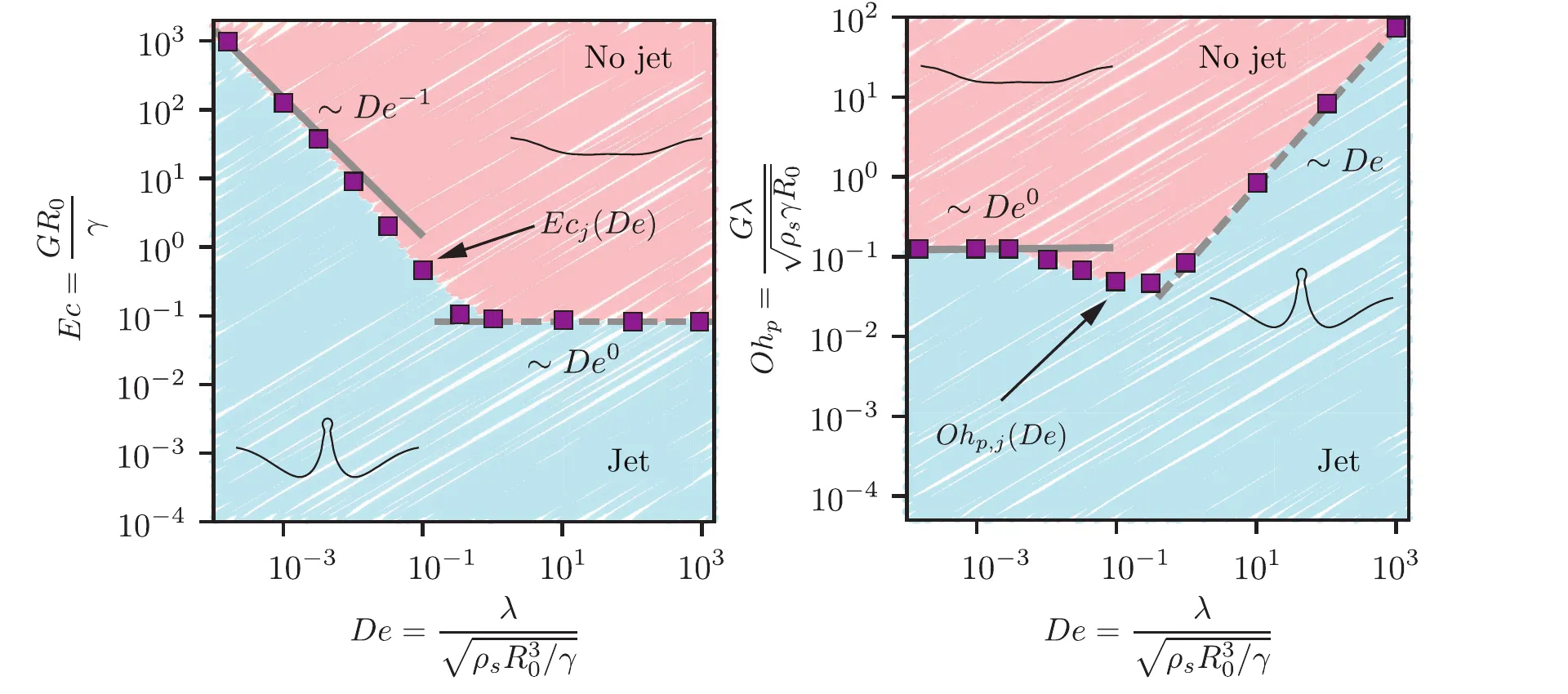Jet versus no jet for a bursting bubble in a viscoelastic liquid. Left: in the plane of the Deborah number and the elastocapillary number . Right: the same boundary in terms of the polymeric Ohnesorge number . Squares mark the simulated boundary; the shaded regions are the jet (blue) and no-jet (pink) regimes. Adapted from Dixit et al. (2025).

The two panels show the same boundary, because

Read the map in two halves. The thresholds below describe the limiting branches of this parameter cut; their values are approximate, not universal.

• Small (fast relaxation). The polymers relax faster than the cavity collapses, so they act only as extra viscosity . The jet disappears once the polymeric Ohnesorge number exceeds about , that is , which in the – plane is the line .
• Large (slow relaxation). The polymers keep their stretch during the collapse and act elastically. Now the elastic stress itself must be small enough: the jet disappears for above about (), which in the other panel is .

Within the jet regime the paper also separates jets that release droplets from jets that do not; for some intermediate values of and the droplets are smaller than in a Newtonian liquid.

2.3 Why the polymers act as viscosity at small

A slender jet obeys a one-dimensional momentum balance (Shi, Brenner & Nagel 1994; Driessen, Jeurissen, Wijshoff, Toschi & Lohse 2013). For the axial velocity and local radius ,

with the interface curvature. The bracket is the tensile stress difference in the jet: the solvent contributes and the polymers .

Integrating over the jet, the momentum of a jet of length changes through the tensile stress at its base. When the polymers relax quickly compared with the local deformation, and , so the polymer contribution is . The base stress is then with an effective extensional viscosity : solvent and polymers both carry the Trouton factor three.

Balancing the jet’s momentum flux against this stress gives , with the jet speed and the length scale at the jet base. If the jet Weber number stays roughly constant across the cases compared, eliminating gives

A constant is an extra scaling assumption, not something the balance itself guarantees.

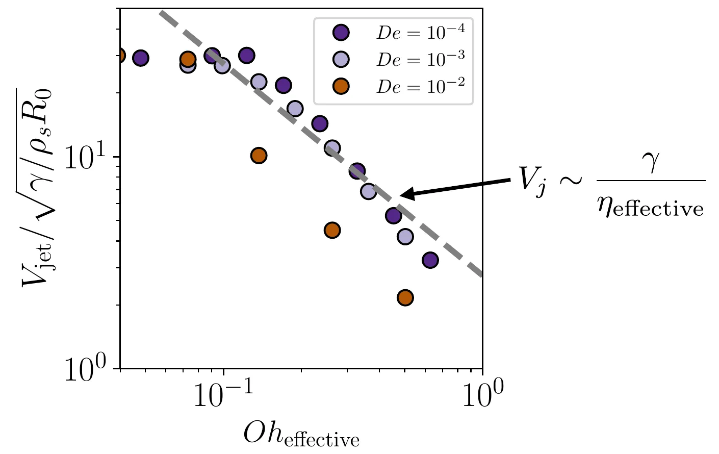Jet speed (in units of ) against an effective Ohnesorge number, for three small Deborah numbers, from the simulations of §2.2. As plotted in the lecture, , which keeps only the axial polymer stress; the full result above, , differs only in the polymer weighting. At and the data follow the inverse-viscosity trend (dashed line) over much of the range; at they fall clearly below it.

2.4 Intermezzo: yield stress

Toothpaste and peanut butter hold their shape until pushed hard enough: they have a yield stress . The bubbling mud pots of Yellowstone (video in Lecture 1) are a yield-stress free-surface flow.

A convenient model is Saramito’s elastoviscoplastic extension of Oldroyd-B (Saramito 2007). Write the polymer stress as , its deviatoric part as , and the equivalent shear stress as . The polymer stress relaxes only once exceeds the yield stress:

• Below the yield stress (, so ) the material is a Kelvin–Voigt solid.
• Far above it () it is a viscoelastic Oldroyd-B liquid.

The new dimensionless group is the plastocapillary number .

When elasticity can be neglected we recover the Bingham viscoplastic model (Eugene C. Bingham, 1878–1945). With the deviatoric extra stress, the norm and built on the plastic viscosity , the dimensionless model is

For a bursting bubble in a viscoplastic medium, recovers the Newtonian case, with capillary waves and a jet. As grows, the driving stresses fall below the yield stress before the cavity has relaxed, and the surface freezes into a non-flat final shape instead of becoming flat again (Sanjay, Lohse & Jalaal 2021). With elasticity included as well (Balasubramanian, Sanjay, Jalaal, Vinuesa & Tammisola 2024), elastic relaxation has a non-monotonic effect on the jet, and plasticity matters mainly when relaxation is fast.

3) Drops: impact forces from Wagner to Hertz

3.1 Liquid drops and elastic beads

A water drop in space bounces off a hydrophobic paddle almost like a ball (liquid ping-pong on the ISS). So how different are a liquid drop and an elastic bead hitting a wall? Consider a sphere of radius and density arriving at speed , on the impact time .

Wagner (liquids). In the early inertial stage the displaced free surface enlarges the contact region: Wagner theory gives , against for the geometric intersection of an undeformed sphere with the wall. The force comes from bringing liquid to rest in this fast-growing foot. At large and small viscosity only inertia enters, so the first force peak scales as .

Hertz (elastic solids). A sphere compressed by , with contact radius , stores elastic energy . Setting this equal to the kinetic energy gives the maximum compression . The contact force then gives the scaling in the table.

3.2 Liquid drops: the first force peak

Force measurements on drops hitting a superhydrophobic surface show two peaks: one at impact and one when the drop jumps off, as a Worthington jet forms inside it (Zhang, Sanjay et al. 2022). The first peak follows inertial scaling:

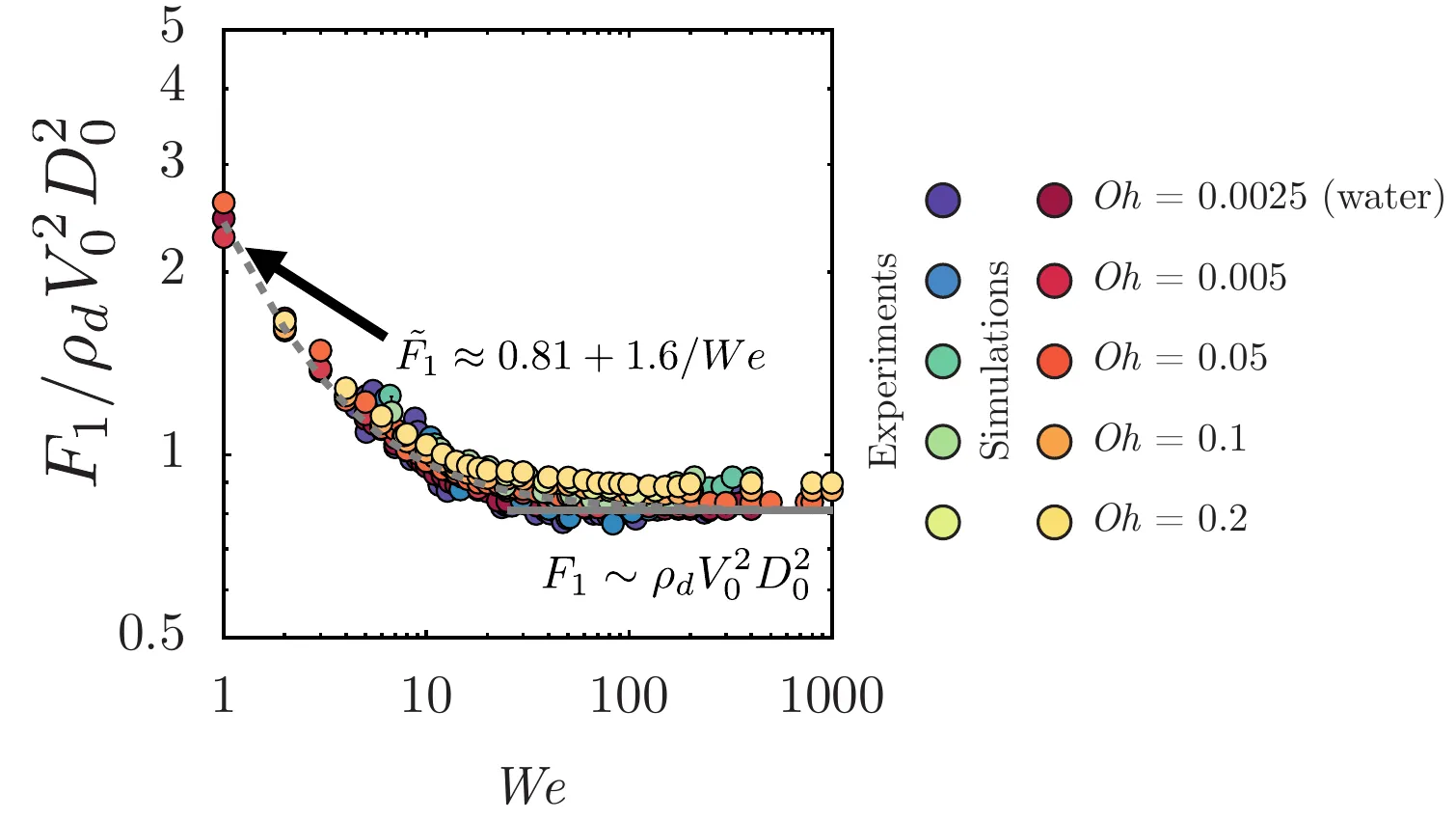First force peak , scaled by , against the Weber number , where is the drop density and the drop diameter. Experiments and simulations span (water) to . The data approximately collapse onto , with modest viscosity-dependent departures (Zhang, Sanjay et al. 2022; Sanjay et al. 2025).

The first peak barely depends on viscosity: it stays the same for liquids up to about a hundred times more viscous than water (Sanjay, Zhang, Lv & Lohse 2025). Only for much more viscous drops does dissipation take over. In terms of the radius, which we use from here on, the peak force is with . At large this tends to the Wagner value ; at small capillarity adds to it. A unified scaling theory for both the impact force and the maximum spreading diameter is given by Sanjay & Lohse (2025).

3.3 From liquid drops to elastic beads

Now give the drop an elastic modulus . For impact the natural memory number is the Weissenberg number , related to the capillary-time Deborah number by (with ). In the infinite-memory limit , and at fixed solvent Ohnesorge number, the force is set by and , or equivalently by and the elasticity number (Jana, Kolinski, Lohse & Sanjay 2026).

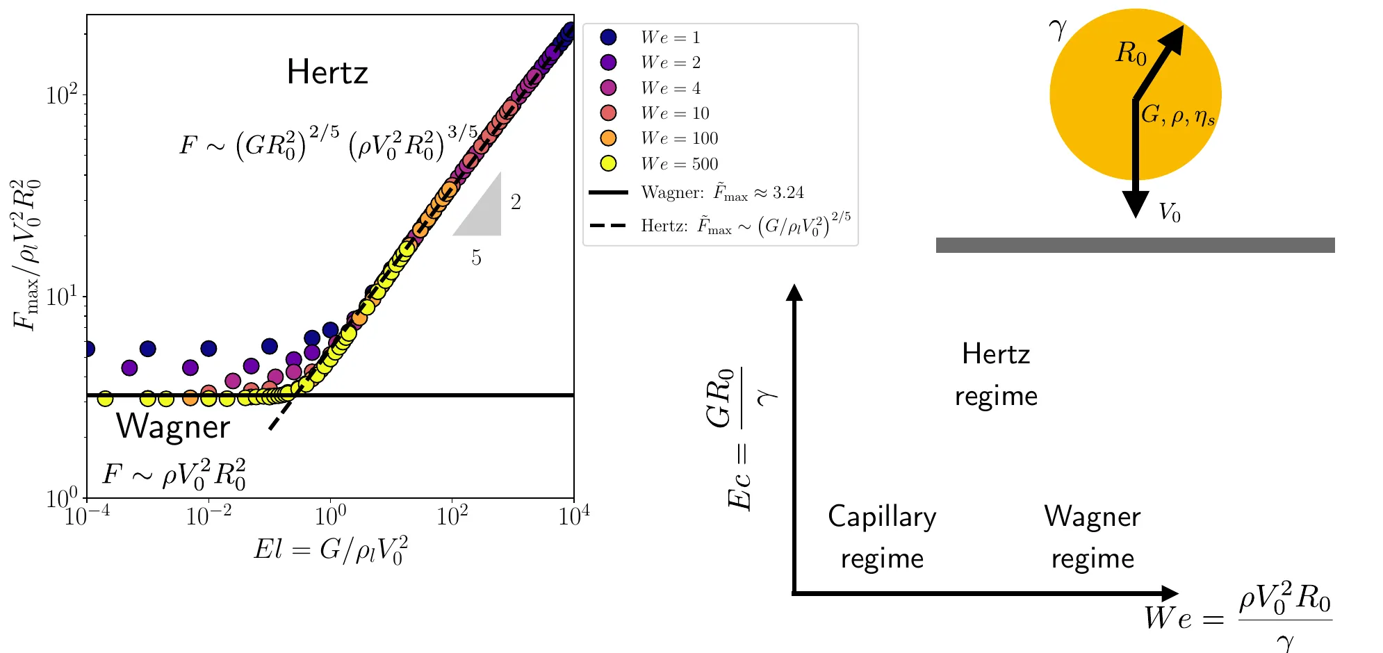Left: peak impact force against the elasticity number at , for Weber numbers from 1 to 500. At small the large- curves approach the Wagner plateau, while smaller keep a capillary contribution; at large the curves approach the Hertz scaling . Right: the resulting regime map in the plane of and , with capillary, Wagner and Hertz regimes. Simulations as in Jana et al. (2026).

• For the sphere behaves like a liquid drop: Wagner, , plus a capillary correction at small .
• For it behaves like an elastic bead: Hertz, . Hertz’s contact theory for an incompressible elastic sphere gives the prefactor ; the simulations give .
• The transition from Wagner to Hertz is smooth, and the force curve changes shape with it: a stiff sphere gives a single, nearly symmetric force pulse, as a bouncing elastic ball does.

Sweeping the relaxation time from zero to infinity takes the same sphere continuously from a liquid drop with no memory to an elastic bead with permanent memory.

Summary

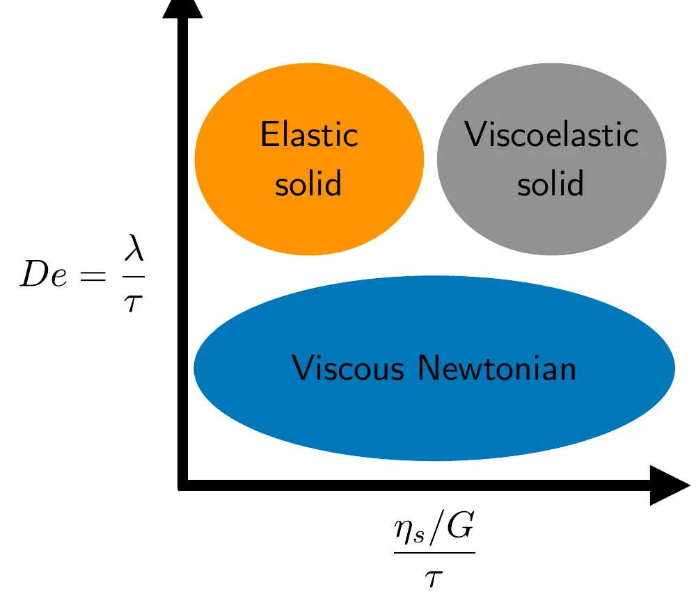Where the three behaviours live, in terms of the Deborah number (relaxation time over flow time) and the retardation time over the flow time .

1. One model, the Oldroyd-B family, covers viscous liquids (), elastic solids (, ) and viscoelastic Kelvin–Voigt solids (, of order one or larger).
2. Sheets: viscous dissipation in a retracting film stays finite as the viscosity vanishes. Elasticity adds a hoop stress that slows the opening and, once is of order one, is expected to stop it.
3. Bubbles: polymers can suppress the Worthington jet. For the parameter cut shown, the jet stops at roughly at small , where the polymers act as extra viscosity, and at roughly at large , where they act elastically. A yield stress can freeze the cavity before it relaxes.
4. Drops: the impact force goes from Wagner, , to Hertz, , as the elasticity number crosses one.

Self-check questions

1. Show that . Use this to explain why the jet/no-jet boundary looks like at small but like at large .
2. In the Kelvin–Voigt limit (), what is for a simple shear of amount , and what is the resulting shear stress?
3. Derive the Hertz scaling from an energy balance, and show that the Wagner and Hertz forces are equal when is of order one.
4. Why is the first force peak of a low-viscosity drop insensitive to viscosity? Compare the impact time with the time for viscous effects to diffuse across the drop.
5. Estimate when elasticity can halt the opening of a hole in a sheet by comparing the elastic stress with the capillary stress .

References

1. D. Tammaro, R. Pasquino, M. M. Villone, G. D’Avino, V. Ferraro, E. Di Maio, A. Langella, N. Grizzuti & P. L. Maffettone, Elasticity in bubble rupture, Langmuir 34, 5646–5654 (2018). doi:10.1021/acs.langmuir.8b00520
2. V. Sanjay, U. Sen, P. Kant & D. Lohse, Taylor–Culick retractions and the influence of the surroundings, J. Fluid Mech. 948, A14 (2022). doi:10.1017/jfm.2022.671
3. J. H. Snoeijer, A. Pandey, M. A. Herrada & J. Eggers, The relationship between viscoelasticity and elasticity, Proc. R. Soc. A 476, 20200419 (2020). doi:10.1098/rspa.2020.0419
4. E. Ghabache, G. Liger-Belair, A. Antkowiak & T. Séon, Evaporation of droplets in a Champagne wine aerosol, Sci. Rep. 6, 25148 (2016). doi:10.1038/srep25148
5. J. M. Cheny & K. Walters, Extravagant viscoelastic effects in the Worthington jet experiment, J. Non-Newtonian Fluid Mech. 67, 125–135 (1996). doi:10.1016/S0377-0257(96)01473-5
6. A. K. Dixit, A. Oratis, K. Zinelis, D. Lohse & V. Sanjay, Viscoelastic Worthington jets and droplets produced by bursting bubbles, J. Fluid Mech. 1010, A2 (2025). doi:10.1017/jfm.2025.237
7. X. D. Shi, M. P. Brenner & S. R. Nagel, A cascade of structure in a drop falling from a faucet, Science 265, 219–222 (1994). doi:10.1126/science.265.5169.219
8. T. Driessen, R. Jeurissen, H. Wijshoff, F. Toschi & D. Lohse, Stability of viscous long liquid filaments, Phys. Fluids 25, 062109 (2013). doi:10.1063/1.4811849
9. P. Saramito, A new constitutive equation for elastoviscoplastic fluid flows, J. Non-Newtonian Fluid Mech. 145, 1–14 (2007). doi:10.1016/j.jnnfm.2007.04.004
10. V. Sanjay, D. Lohse & M. Jalaal, Bursting bubble in a viscoplastic medium, J. Fluid Mech. 922, A2 (2021). doi:10.1017/jfm.2021.489
11. A. G. Balasubramanian, V. Sanjay, M. Jalaal, R. Vinuesa & O. Tammisola, Bursting bubble in an elastoviscoplastic medium, J. Fluid Mech. 1001, A9 (2024). doi:10.1017/jfm.2024.1073
12. B. Zhang, V. Sanjay, S. Shi, Y. Zhao, C. Lv, X.-Q. Feng & D. Lohse, Impact forces of water drops falling on superhydrophobic surfaces, Phys. Rev. Lett. 129, 104501 (2022). doi:10.1103/PhysRevLett.129.104501
13. V. Sanjay, B. Zhang, C. Lv & D. Lohse, The role of viscosity on drop impact forces on non-wetting surfaces, J. Fluid Mech. 1004, A6 (2025). doi:10.1017/jfm.2024.982
14. V. Sanjay & D. Lohse, Unifying theory of scaling in drop impact: forces and maximum spreading diameter, Phys. Rev. Lett. 134, 104003 (2025). doi:10.1103/PhysRevLett.134.104003
15. S. Jana, J. Kolinski, D. Lohse & V. Sanjay, Impacting spheres: from liquid drops to elastic beads, Soft Matter 22, 2226–2236 (2026). doi:10.1039/D5SM01078K

Previous Lecture: Lecture 5: Elastic vs Viscous vs Viscoelastic
Next Lecture: Lectures 7-8: Student Presentations
Course Home: Course Overview

Metadata

Author:: Vatsal Sanjay
Date published:: Jul 19, 2026
Date modified:: Oct 15, 2026

Back to main website

Home, Team, Research, Github

📝 Edit this page on GitHub